An end-to-end machine learning workflow can be broken down into many steps, and there are an extensive number of layers of complexity that can be added, serving a variety of purposes. However, in this guide we will work through a bare bones workflow, using a simple dataset, in order to get a better understanding of the process.
A simple end-to-end ML solution will typically include the following steps:
Though in this instance, the data is relatively clean, the following steps are included to demonstrate how you might clean data in a real-world scenario. Dropping NAs and duplicates should, however, be done with care (see discussion below).
# check for missing valuesdf.isna().sum()# drop missing valuesdf.dropna(inplace=True)# check for duplicatesdf.duplicated().sum()# drop duplicatesdf.drop_duplicates(inplace=True)
There are several variables for which there appear to be missing values in the form of zeroes. This was identified in the exploratory data analysis notebook in this project. Variables like cholesterol and resting_bp should not be zero, and because the target class is disproportionately distributed within these zero values, it is important to address the problem.
There are a number of choices that could be made when it comes to dealing with null or missing values, and there are robust approaches to imputation (though it is necessary to take great care when doing so), however in the interest of simplicity, we will simply remove the rows with zero values in this instance.1
# remove zero valuesdf = df[(df['cholesterol'] !=0) & (df['resting_bp'] !=0)]
8.1.2 Train/Test Split
One of the central tenets of machine learning is that the model should not be trained on the same data that it is evaluated on. This is because the model could learn spurious/random patterns and correlations in the training data, and this will harm the model’s ability to make good predictions on new, unseen data. There are many way of trying to resolve this, but the most simple approach is to split the data into a training and test set. The training set will be used to train the model, and the test set will be used to evaluate the model.
# split data into train and test setsX = df.drop('heart_disease', axis=1)y = df['heart_disease']X_train, X_test, y_train, y_test = train_test_split(X, y, test_size=0.2, random_state=123)
8.1.3 Preprocessing
The purpose of preprocessing is to prepare the data for model fitting. This can take a number of different forms, but some of the most common preprocessing steps include:
Normalising/Standardising data
One-hot encoding categorical variables
Removing outliers
Imputing missing values
We will build a preprocessing recipe that one-hot encodes all categorical features, and normalises the numeric features so that they have a mean of zero and a standard deviation of one.
# specify all features for the modelfeats = df.drop('heart_disease', axis=1)# specify targettarget = ['heart_disease']# get categorical columnscat_cols = df.select_dtypes(include='object').columns# get numerical columns (excluding target)num_cols = df.drop('heart_disease', axis=1).select_dtypes(exclude='object').columnsscaler = Pipeline(steps=[('scaler', StandardScaler())])one_hot = Pipeline(steps=[('one_hot', OneHotEncoder(drop='first'))])preprocess = ColumnTransformer( transformers=[ ('nums', scaler, num_cols), ('cats', one_hot, cat_cols) ])
8.2 Model Training
There are many different types of models that can be used for classification problems, and selecting the right model for the problem at hand can be difficult when you are first starting out with machine learning.
Simple models like linear and logistic regressions are often a good place to start and can be used to get a better understanding of the data and the problem at hand, and can give you a good idea of baseline performance before building more complex models to improve performance. Another example of a simple model is K-Nearest Neighbours (KNN), which is a non-parametric model that can be used for both classification and regression problems.
We will fit a logistic regression and a KNN, as well as fitting a Random Forest model, which is a good example of a slightly more complex model that will often perform well on structured data.
8.2.1 Cross-Validation
On top of the train/test split, we will also use cross-validation to train our models. Cross-validation is a method of training a model on a subset of the data, and then evaluating the model on the remaining data. This process is repeated multiple times, and the average performance is used to evaluate the model. This helps make the training process more generalisable.
For more information on cross-validation and how it can be used to train models:
The Cross-Validation section in the Scikit-learn documentation provides a good overview of cross-validation and how it can be used to train models. It includes a discussion of a typical cross-validation workflow; the different types of cross-validation, their implementation in Scikit-learn, and their pros and cons; and the documentation is accompanied by a lot of really helpful visuals.
Neptune AI’s blog post on cross-validation goes into detail discussing cross-validation strategies, and gives clear visual demonstrations of how each strategy works.
We will use 5-fold stratified cross-validation to train our models. This means that the training data will be split into 5 folds, ensuring that each fold has the same proportion of the target classes. Each fold will be used as a test set once, and the remaining folds will be used as training sets. This will be repeated 5 times, and the average performance will be used to evaluate the model.
Although the logistic regression performs slightly better than the random forest, the random forest has higher standard deviation and has more hyperparameters that can be tuned, so it is likely this will model has the highest potential.
8.2.2 Hyperparameter Tuning
Having defined the preprocessing pipeline, we can now train and tune the models. We will use the GridSearchCV() function to carry out hyperparameter tuning[^tuning], which will search over a grid of hyperparameter values (specified by params) to find the best performing model. We will use 5-fold cross-validation to train the models, and will evaluate the models using F1 score and accuracy.
For a more detailed discussion of hyperparameter tuning, and the different methods for tuning in Scikit-learn, the Tuning the Hyperparameters of an Estimator section of the Scikit-learn documentation is a good place to start, and the Hyperparameter Tuning by Grid Search section of the Scikit-learn course is an excellent accompaniment.
In addition, the AWS overview of hyperparameter tuning is a good resource if you are only looking for a brief overview. For an in-depth discussion about how hyperparameter tuning works, including the mathematics behind it, Jeremy Jordan’s Hyperparameter Tuning for Machine Learning Models blogpost is thorough but easy to follow.
There are a lot of different Python libraries for hyperparameter tuning, however the most popular libraries that are specifically designed for tuning are Hyperopt and Optuna. Both can be used to tune models built with Scikit-learn (and many other frameworks) and can often produce better results than Scikit-learn’s built-in hyperparameter tuning methods. I have had limited experience using Hyperopt, however I have used Optuna often and I would highly recommend it if/when you are ready to move beyond Scikit-learn’s options for tuning.
params = { 'rf__bootstrap': [True],'rf__max_depth': [10, 20, 30],"rf__min_samples_leaf" : [1, 2, 4],"rf__min_samples_split" : [2, 5, 10],"rf__n_estimators": [100, 250, 500] }pipeline = Pipeline([ ('preprocess', preprocess), ('rf', RandomForestClassifier(random_state=123))])clf = GridSearchCV( estimator=pipeline, param_grid=params, scoring='f1', cv=kf, verbose=1, refit=True )# tune random foresttuning_results = clf.fit(X_train, y_train)# get the f1 score for training setprint('Training F1 Score: %.2f'% (tuning_results.best_score_))# get the best performing model on training setbest_model = tuning_results.best_estimator_
Fitting 5 folds for each of 81 candidates, totalling 405 fits
Training F1 Score: 0.79
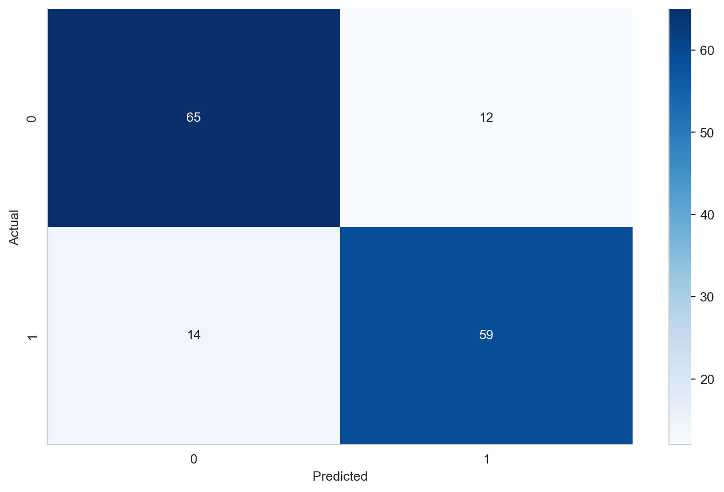
8.3 Model Evaluation
# get predictions on holdout setpreds = best_model.predict(X_test)# get the f1 score for holdout setsprint('Holdout F1 Score: %.2f'% (f1_score(y_test, preds)))
For a guided video course, Data Talks Club’s Machine Learning Zoomcamp (available on Github and Youtube) is well-paced and well-presented, covering a variety of machine learning methods and even covering some of the aspects that introductory course often skip over, like deployment and data engineering principles. However, while the ML Zoomcamp course is intended as an introduction to machine learning, it does assume a certain level of familiarity with programming (the course uses Python) and software engineering. The appendix section of the course is definitely helpful for bridging some of the gaps in the course, but it is still worth being aware of the way the course is structured.
If you are looking for something that goes into greater detail about a wide range of machine learning methods, then there is no better resource than An Introduction to Statistical Learning (or its accompanying online course), by Gareth James, Daniela Witten, Trevor Hastie, and Robert Tibshirani.
Finally, if you are particularly interested in learning the mathematics that underpins machine learning, I would highly recommend Mathematics of Machine Learning, which is admittedly not free but is very, very good. If you want to learn about the mathematics of machine learning but are not comfortable enough tackling the Mathematics of ML book, the StatQuest and 3Blue1Brown Youtube channels are both really accessible and well-presented.
In a real-world analysis, it would be important to understand why the data is missing, and to consider the implications of removing the data. For example, if the data is missing at random, then removing the data will not have a significant impact on the analysis. However, if the data is missing because it was not collected, or if the data is missing because it is not available, then removing the data could have a significant impact on the analysis.↩︎
Source Code
# End-to-End Machine Learning Workflow {#sec-ml-workflow}```{python}#| label: setup#| code-fold: true#| code-summary: 'Setup Code (Click to Expand)'# import librariesimport pandas as pdimport numpy as npimport matplotlib.pyplot as pltimport seaborn as snsfrom matplotlib import rcfrom sklearn.compose import ColumnTransformerfrom sklearn.ensemble import RandomForestClassifierfrom sklearn.linear_model import LogisticRegressionfrom sklearn.metrics import confusion_matrixfrom sklearn.metrics import f1_scorefrom sklearn.model_selection import cross_val_scorefrom sklearn.model_selection import GridSearchCVfrom sklearn.model_selection import StratifiedKFoldfrom sklearn.model_selection import train_test_splitfrom sklearn.neighbors import KNeighborsClassifierfrom sklearn.pipeline import make_pipeline, Pipelinefrom sklearn.preprocessing import OneHotEncoder, StandardScaler# import datadf = pd.read_csv("https://raw.githubusercontent.com/NHS-South-Central-and-West/data-science-guides/main/data/heart_disease.csv")# set plot stylesns.set_style('whitegrid')# set plot fontrc('font',**{'family':'sans-serif','sans-serif':['Arial']})# set plot colour palettecolours = ['#1C355E', '#00A499', '#005EB8']sns.set_palette(sns.color_palette(colours))```An end-to-end machine learning workflow can be broken down into many steps, and there are an extensive number of layers of complexity that can be added, serving a variety of purposes. However, in this guide we will work through a bare bones workflow, using a simple dataset, in order to get a better understanding of the process.A simple end-to-end ML solution will typically include the following steps:1. Importing & Cleaning Data2. Exploratory Data Analysis (See @sec-eda)3. Data Preprocessing4. Model Training - Selecting from Candidate Models - Hyperparameter Tuning - Identifying Best Model5. Fitting Model on Test Data6. Model Evaluation## Data```{python}#| label: data_summary# data summarydf.info()df.describe()df.head()```### CleaningThough in this instance, the data is relatively clean, the following steps are included to demonstrate how you might clean data in a real-world scenario. Dropping NAs and duplicates should, however, be done with care (see discussion below).```{python}#| label: data_cleaning# check for missing valuesdf.isna().sum()# drop missing valuesdf.dropna(inplace=True)# check for duplicatesdf.duplicated().sum()# drop duplicatesdf.drop_duplicates(inplace=True)```There are several variables for which there appear to be missing values in the form of zeroes. This was identified in the exploratory data analysis notebook in this project. Variables like `cholesterol` and `resting_bp` should not be zero, and because the target class is disproportionately distributed within these zero values, it is important to address the problem.There are a number of choices that could be made when it comes to dealing with null or missing values, and there are robust approaches to imputation (though it is necessary to take great care when doing so), however in the interest of simplicity, we will simply remove the rows with zero values in this instance.[^1][^1]: In a real-world analysis, it would be important to understand why the data is missing, and to consider the implications of removing the data. For example, if the data is missing at random, then removing the data will not have a significant impact on the analysis. However, if the data is missing because it was not collected, or if the data is missing because it is not available, then removing the data could have a significant impact on the analysis.```{python}#| label: remove-zero-values# remove zero valuesdf = df[(df['cholesterol'] !=0) & (df['resting_bp'] !=0)]```### Train/Test SplitOne of the central tenets of machine learning is that the model should not be trained on the same data that it is evaluated on. This is because the model could learn spurious/random patterns and correlations in the training data, and this will harm the model's ability to make good predictions on new, unseen data. There are many way of trying to resolve this, but the most simple approach is to split the data into a training and test set. The training set will be used to train the model, and the test set will be used to evaluate the model.```{python}#| label: train_test_split# split data into train and test setsX = df.drop('heart_disease', axis=1)y = df['heart_disease']X_train, X_test, y_train, y_test = train_test_split(X, y, test_size=0.2, random_state=123)```### PreprocessingThe purpose of preprocessing is to prepare the data for model fitting. This can take a number of different forms, but some of the most common preprocessing steps include:- Normalising/Standardising data- One-hot encoding categorical variables- Removing outliers- Imputing missing valuesWe will build a preprocessing recipe that one-hot encodes all categorical features, and normalises the numeric features so that they have a mean of zero and a standard deviation of one.```{python}#| label: preprocessing# specify all features for the modelfeats = df.drop('heart_disease', axis=1)# specify targettarget = ['heart_disease']# get categorical columnscat_cols = df.select_dtypes(include='object').columns# get numerical columns (excluding target)num_cols = df.drop('heart_disease', axis=1).select_dtypes(exclude='object').columnsscaler = Pipeline(steps=[('scaler', StandardScaler())])one_hot = Pipeline(steps=[('one_hot', OneHotEncoder(drop='first'))])preprocess = ColumnTransformer( transformers=[ ('nums', scaler, num_cols), ('cats', one_hot, cat_cols) ])```## Model TrainingThere are many different types of models that can be used for classification problems, and selecting the right model for the problem at hand can be difficult when you are first starting out with machine learning.Simple models like [linear](https://scikit-learn.org/stable/modules/generated/sklearn.linear_model.LinearRegression.html) and [logistic](https://scikit-learn.org/stable/modules/generated/sklearn.linear_model.LogisticRegression.html) regressions are often a good place to start and can be used to get a better understanding of the data and the problem at hand, and can give you a good idea of baseline performance before building more complex models to improve performance. Another example of a simple model is [K-Nearest Neighbours](https://scikit-learn.org/stable/modules/generated/sklearn.neighbors.KNeighborsClassifier.html) (KNN), which is a non-parametric model that can be used for both classification and regression problems.We will fit a logistic regression and a KNN, as well as fitting a Random Forest model, which is a good example of a slightly more complex model that will often perform well on structured data.### Cross-ValidationOn top of the train/test split, we will also use cross-validation to train our models. Cross-validation is a method of training a model on a subset of the data, and then evaluating the model on the remaining data. This process is repeated multiple times, and the average performance is used to evaluate the model. This helps make the training process more generalisable.For more information on cross-validation and how it can be used to train models:- The [Cross-Validation](https://scikit-learn.org/stable/modules/cross_validation.html) section in the Scikit-learn documentation provides a good overview of cross-validation and how it can be used to train models. It includes a discussion of a typical cross-validation workflow; the different types of cross-validation, their implementation in Scikit-learn, and their pros and cons; and the documentation is accompanied by a lot of really helpful visuals.- Neptune AI's [blog post](https://neptune.ai/blog/cross-validation-in-machine-learning-how-to-do-it-right) on cross-validation goes into detail discussing cross-validation strategies, and gives clear visual demonstrations of how each strategy works.We will use 5-fold stratified cross-validation to train our models. This means that the training data will be split into 5 folds, ensuring that each fold has the same proportion of the target classes. Each fold will be used as a test set once, and the remaining folds will be used as training sets. This will be repeated 5 times, and the average performance will be used to evaluate the model.```{python}# select models = []models.append(('log', LogisticRegression(random_state=123)))models.append(('knn', KNeighborsClassifier()))models.append(('rf', RandomForestClassifier(random_state=123)))# evaluate each model in turnresults = []names = []n_splits =5for name, model in models: kf = StratifiedKFold(n_splits, random_state=123, shuffle=True) pipeline = Pipeline([ ('preprocess', preprocess), ('model', model) ]) cv_scores = cross_val_score( pipeline, X_train, y_train, cv=kf, scoring='f1' ) results.append(cv_scores) names.append(name)print('%s: %.2f (%.3f)'% (name, cv_scores.mean(), cv_scores.std()))```Although the logistic regression performs slightly better than the random forest, the random forest has higher standard deviation and has more hyperparameters that can be tuned, so it is likely this will model has the highest potential.### Hyperparameter TuningHaving defined the preprocessing pipeline, we can now train and tune the models. We will use the `GridSearchCV()` function to carry out hyperparameter tuning[^tuning], which will search over a grid of hyperparameter values (specified by `params`) to find the best performing model. We will use 5-fold cross-validation to train the models, and will evaluate the models using F1 score and accuracy.For a more detailed discussion of hyperparameter tuning, and the different methods for tuning in Scikit-learn, the [Tuning the Hyperparameters of an Estimator](https://scikit-learn.org/stable/modules/grid_search.html#) section of the Scikit-learn documentation is a good place to start, and the [Hyperparameter Tuning by Grid Search](https://inria.github.io/scikit-learn-mooc/python_scripts/parameter_tuning_grid_search.html) section of the Scikit-learn course is an excellent accompaniment.In addition, the AWS overview of [hyperparameter tuning](https://docs.aws.amazon.com/sagemaker/latest/dg/automatic-model-tuning-how-it-works.html) is a good resource if you are only looking for a brief overview. For an in-depth discussion about how hyperparameter tuning works, including the mathematics behind it, Jeremy Jordan's [Hyperparameter Tuning for Machine Learning Models](https://www.jeremyjordan.me/hyperparameter-tuning/) blogpost is thorough but easy to follow.There are a lot of different Python libraries for hyperparameter tuning, however the most popular libraries that are specifically designed for tuning are [Hyperopt](http://hyperopt.github.io/hyperopt/) and [Optuna](https://optuna.org/). Both can be used to tune models built with Scikit-learn (and many other frameworks) and can often produce better results than Scikit-learn's built-in hyperparameter tuning methods. I have had limited experience using Hyperopt, however I have used Optuna often and I would highly recommend it if/when you are ready to move beyond Scikit-learn's options for tuning.```{python}params = { 'rf__bootstrap': [True],'rf__max_depth': [10, 20, 30],"rf__min_samples_leaf" : [1, 2, 4],"rf__min_samples_split" : [2, 5, 10],"rf__n_estimators": [100, 250, 500] }pipeline = Pipeline([ ('preprocess', preprocess), ('rf', RandomForestClassifier(random_state=123))])clf = GridSearchCV( estimator=pipeline, param_grid=params, scoring='f1', cv=kf, verbose=1, refit=True )# tune random foresttuning_results = clf.fit(X_train, y_train)# get the f1 score for training setprint('Training F1 Score: %.2f'% (tuning_results.best_score_))# get the best performing model on training setbest_model = tuning_results.best_estimator_```## Model Evaluation```{python}#| label: evaluation# get predictions on holdout setpreds = best_model.predict(X_test)# get the f1 score for holdout setsprint('Holdout F1 Score: %.2f'% (f1_score(y_test, preds)))``````{python}#| label: confusion-matrix# get confusion matrixconf_mat = pd.crosstab(y_test, preds, rownames=['Actual'], colnames=['Predicted'])# plot confusion matrixfig, ax = plt.subplots()sns.heatmap( data = conf_mat, annot=True, cmap='Blues', fmt='g' )sns.despine()plt.show()```## Model InterpretationWe can compute the features that are most important in predicting heart disease.```{python}#| label: feature-importance# get feature importancefeature_importance = best_model.named_steps['rf'].feature_importances_# get feature namesfeature_names = ( best_model .named_steps['preprocess'] .transformers_[1][1] .named_steps['one_hot'] .get_feature_names_out(cat_cols) .tolist())# get feature namesfeature_names = num_cols.tolist() + feature_names# create dataframefeat_importance = pd.DataFrame({'feature': feature_names, 'importance': feature_importance })# plot feature importancefig, ax = plt.subplots()sns.barplot( x='importance', y='feature', data=feat_importance.sort_values(by='importance', ascending=False), color='#1C355E' )sns.despine()plt.show()```## Next Steps## ResourcesThere are lots of great (and free) introductory resources for machine learning:- [Machine Learning University](https://aws.amazon.com/machine-learning/mlu)- [MLU Explain](https://mlu-explain.github.io/)- [Machine Learning for Beginners](https://microsoft.github.io/ML-For-Beginners/?utm_source=substack&utm_medium=email#/)For a guided video course, Data Talks Club's Machine Learning Zoomcamp (available on [Github](https://github.com/alexeygrigorev/mlbookcamp-code/tree/master/course-zoomcamp) and [Youtube](https://www.youtube.com/watch?v=MqI8vt3-cag&list=PL3MmuxUbc_hIhxl5Ji8t4O6lPAOpHaCLR)) is well-paced and well-presented, covering a variety of machine learning methods and even covering some of the aspects that introductory course often skip over, like deployment and data engineering principles. However, while the ML Zoomcamp course is intended as an introduction to machine learning, it does assume a certain level of familiarity with programming (the course uses Python) and software engineering. The appendix section of the course is definitely helpful for bridging some of the gaps in the course, but it is still worth being aware of the way the course is structured.If you are looking for something that goes into greater detail about a wide range of machine learning methods, then there is no better resource than [An Introduction to Statistical Learning](https://hastie.su.domains/ISLR2/ISLRv2_website.pdf) (or its accompanying [online course](https://www.statlearning.com/online-course)), by Gareth James, Daniela Witten, Trevor Hastie, and Robert Tibshirani.Finally, if you are particularly interested in learning the mathematics that underpins machine learning, I would highly recommend [Mathematics of Machine Learning](https://tivadardanka.com/books/mathematics-of-machine-learning), which is admittedly not free but is very, very good. If you want to learn about the mathematics of machine learning but are not comfortable enough tackling the Mathematics of ML book, the [StatQuest](https://www.youtube.com/channel/UCtYLUTtgS3k1Fg4y5tAhLbw) and [3Blue1Brown](https://www.youtube.com/c/3blue1brown) Youtube channels are both really accessible and well-presented.